Did water saving irrigation protect water resources over the past 40 years

A R T I C L E I N F O

Handling Editor - Dr Z Xiying

Keywords:

Paradox of irrigation efficiency Water accounting framework Water savings estimation Satellite-based ET partitions

A B S T R A C T

Water-saving technologies have long been seen as an effective method to reduce irrigation water use and alle- viate regional water shortage. However, growing reports of more severe water shortage and increasing appli- cation of water-saving technologies across the world have necessitated reassessment of agricultural water-saving. This study develops a simple method based on satellite-based ET partitions to estimate water withdrawal, water consumption and return flow from the 1980s to 2010s, and quantifies water-savings across globe and four hot- spot irrigated areas at both field and regional scales based on water accounting framework. The results show that global irrigation water flows keep increasing from the 1980s to 2010s, with over 50% increase from the expansion in irrigated lands. While water-saving technologies are found mainly applied in originally old irrigated lands, traditional flooding irrigation is still dominant in newly-developed irrigated lands. Non-beneficial water consumption (soil evaporation) is effectively reduced by water-saving technologies, but return flow has increased at the same time. At field scale, water-saving technologies fail to save water because the accumulated increased return flow is more than the accumulated decreased non-beneficial water consumption. At regional scale, however, water is saved because the return flow percolated to fresh aquifers is seen as beneficial rather than loss. At the same time, the accumulated increase of beneficial water consumption (crop transpiration) exceeds regional water savings, which explains the paradox between wide application of water-saving technologies and more severe regional water shortage. This study provides key new evidence for the paradox of irrigation effi- ciency and helps reconsidering water-saving technologies and their impacts on regional water resources.

1. Introduction

Irrigation is widely considered a major contributor to water scarcity as it is the largest freshwater user with a long criticism of low efficiency, especially in water-scarce regions (Perry et al., 2009). Thus, water-saving irrigation that aims to reduce inefficient water use and maximizes beneficial crop water use is seen as a basic solution to water scarcity (Perry et al., 2017). Paradoxically, increase in water scarcity has

become common with the growing application of water-saving irriga- tion in recent decades due to the reuse of saved water in the cultivation of more areas, higher crop density and more water-intensive crops (Kendy et al., 2004; Ward and Pulido-Velazquez, 2008; Scott et al., 2014; Fishman et al., 2015; Molle and Tanouti, 2017; Berbel et al., 2018; Grafton et al., 2018). This has changed the current understanding of water-saving and moved water-saving calculations from field scale to region scale. Thus, a scheme called water accounting has been proposed

* Corresponding author.

** Corresponding author at: Key Laboratory of Agricultural Water Resources, Hebei Laboratory of Agricultural Water-Saving, Center for Agricultural Resources Research, Institute of Genetics and Developmental Biology, Chinese Academy of Sciences, Shijiazhuang 050021, China.

E-mail addresses: zhouxy@sjziam.ac.cn (X. Zhou), yonghui.yang@sjziam.ac.cn (Y. Yang).

https://doi.org/10.1016/j.agwat.2021.106793

Received 15 July 2020; Received in revised form 25 December 2020; Accepted 31 January 2021

Available online 17 February 2021

0378-3774/© 2021 Elsevier B.V. All rights reserved.

to reassess irrigation water-saving at regional scale based on the new definition of water flows (Perry, 2007; Gleick et al., 2011; Batchelor et al., 2017).

In water accounting framework, irrigation water use is divided into four parts — i) the beneficial water consumption such as transpiration for crop growth; ii) the non-beneficial water consumption such as

Table 1

A list of the datasets used in this study. Note Agric denotes agriculture, SR de- notes spatial resolution, TR denotes temporal resolution, BIE represents bene- ficial irrigation efficiency, IL is irrigated lands.             

Item Name Period SR (◦) TR

GLEAM 1980–2018 0.25 Monthly

evaporation from bare soil and weed transpiration; iii) the recoverable ET

return flow including water re-entering river, reservoirs and fresh

PML 1981–2012 0.5 Monthly

NTSG 1982–2013 0.083 Monthly

aquifers; iv) the non-recoverable return flow such as percolation to sa- line aquifers or outflow to the ocean (Perry, 2007). At region scale, recoverable return flow can be reused by other users, thus only non-beneficial water consumption and non-recoverable return flow can be seen as a loss. Compared to traditional field-scale framework in that all return flow is seen as loss, the new framework takes more water users into consideration thus calls for a regional-scale reassessment of water savings for irrigation. Although this framework has been successfully applied in some case studies (Vardon et al., 2007; Karimi et al., 2013a, b), however, global assessment of irrigation water-saving at region scale that is based on water accounting framework has not been conducted so far.

Agro-hydrological models have traditionally been used to estimate global irrigation water use (Shiklomanov, 2000; Wada et al., 2011, 2014; Kummu et al., 2016; Chen et al., 2019). However, it is hard to analyze global irrigation water-saving at region scale that is based on water accounting framework through traditional agro-hydrological models. This is because: 1) a lot of studies estimate global irrigation in a certain year or a short time period for a fixed irrigated area, which hampers assessment of the effect of land expansion on irrigation (Hanasaki et al., 2006, 2010; Siebert and Dӧll, 2010). 2) Most agro-hydrological models only calculate net irrigation requirements without accounting for return flow, which is critical for assessing regional water-saving (Dӧll and Siebert, 2002; Haddeland et al., 2006; Siebert and Dӧll, 2010; Haddeland et al., 2014; Müller et al., 2019). 3) For those models that do consider deep percolation, irrigation systems (surface, sprinkler and drip) are insufficiently represented due to the coarse knowledge on irrigation systems, despite their large impact on return flow and groundwater recharge (Hanasaki et al., 2010; Wada et al., 2014; Chen et al., 2019).

Recent boom in partitioned satellite-based evapotranspiration (ET)

products (those partitioning ET into evaporation and transpiration) provides a chance to assess water-saving at both field and region scales based on water accounting framework (Stoy et al., 2019). In this study a simple approach was proposed to estimate irrigation water use (water withdrawal, water consumption and return flow) and divide them into

four components — beneficial and non-beneficial water consumption,

recoverable and non-recoverable return flow using satellite-based ET partitions and other agricultural datasets (Jӓgermeyr et al., 2015; Sie- bert et al., 2015). The novelties of this study include: 1) solving the difficulty of return flow estimation from irrigation using a simple method; and 2) answering how much irrigation water is saved across the globe at both field and region scales. For solving these issues, we setup in this study the following objectives: 1) estimation of water withdrawal, water consumption and return flow from the 1980s to 2010s across the globe and four hot-spot irrigation areas; and (2) investigation of water-saving from irrigation at field and region scales in the past four decades. The results of the study will strengthen our understanding about the change in irrigation across the globe and provide different perspectives on water governance.

2. Data and methodology

2.1. Data

Three partitioned satellite-based ET products, two precipitation datasets, the extent of irrigated lands (HID) and Beneficial Irrigation efficiency (BIE) were used to estimate water withdrawal, water

CRU 1980–2018 0.5 Monthly

GPCC 1980–2016 0.5 Monthly

HID (IL) 1980–2005 0.083 Every five years BIE 1980–2009 0.5 Mean

consumption and return flow for irrigation. The spatiotemporal resolu- tions of these datasets were listed in Table 1 and brief descriptions were provided afterwards.

2.1.1. Satellite-based ET partitions

Global Land Evaporation Amsterdam Model (GLEAM): GLEAM uses the Priestley-Taylor approach to estimate potential evapotranspiration (PET, Miralles et al., 2011; Martens et al., 2017; Appendix A). The es- timates of PET are converted into actual transpiration or bare soil evaporation using a cover-dependent multiplicative stress factor S, ranging within 0 and 1. Validation studies against eddy covariance data

at daily timescales show that the range of average correlations is typi- cally 0.81–0.86 (Martens et al., 2017). GLEAM dataset is openly avail- able at www.gleam.eu.

2.1.1.1. Penman-Monteith-Leuning equation (PML). PML uses the Penman-Monteith model to estimate ET by modeling conductance terms, thus is considered a biophysically sound and robust framework for understanding eco-hydrologic links (Zhang et al., 2010a, 2010b, 2017; Appendix A). The critical parameter of surface conductance Gs is determined by LAI, accounting for stomatal conductance sensitivity to absorbed photosynthetically active radiation and water vapor deficit. Daily validation using 15 global FLUXNET sites shows that the model can explain 73% of the variance in observed ET (Leuning et al., 2008). PML dataset is openly available at https://data.csiro.au/.

2.1.1.2. Numerical Terra-dynamic Simulation Group (NTSG). NTSG also uses PM equation to estimate ET. Alternatively, the normalized differ- ence vegetation index (NDVI) is used to calculate surface conductance to avoid model-related LAI errors (Zhang et al., 2009, 2010a, 2010b;

Appendix A). Globally, the measured and simulated ET agree favorably at daily, monthly and annual time scales with R2 > 0.8 (Zhang et al., 2010a, 2010b). NTSG dataset is available in the public domain at www.

ntsg.umt.edu.

2.1.2. Other gridded products

Climate Research Unit (CRU) and Global Precipitation Climatology Centre (GPCC): Two precipitation datasets, CRU TS v4.03 and GPCC v2018 were used to estimate water consumption and water withdrawal due to long temporal coverage and high spatial resolution. CRU pre- cipitation is available at: https://crudata.uea.ac.uk/cru/data/hrg/cru

_ts_4.03/ and GPCC precipitation available at: https://www.esrl.noaa. gov/psd/data/gridded/data.gpcc.html.

2.1.2.1. Historical Irrigation Dataset (HID). Siebert et al. (2015) collected sub-national statistics of the area equipped for irrigation (AEI) and downscaled the statistics into eight gridded products of time series of AEI from 1900 to 2005. Here, the final version from HYDE source involving only irrigated lands was used. HID is available at https:// mygeohub.org/publications/8/2. The validation of HID dataset through comparison with other products was given in Appendix B.

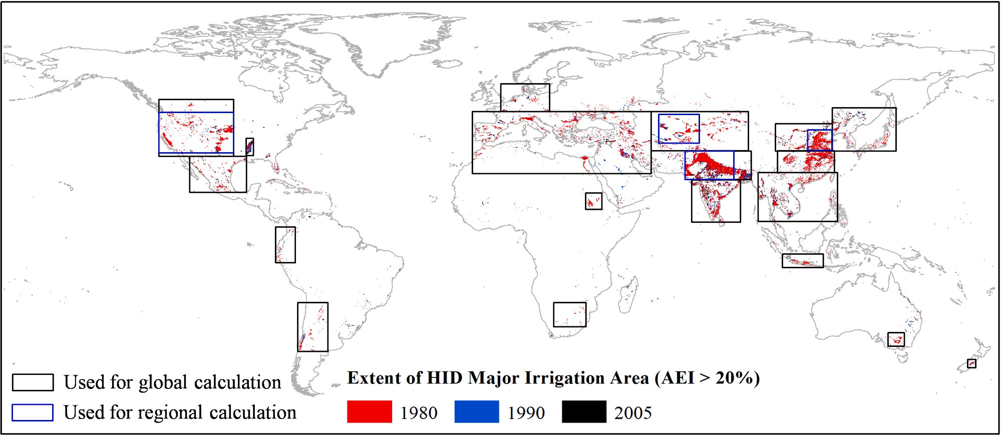
Fig. 1. The spatial distribution of Major Irrigation Areas (MIA) and the domains used for global (black rectangles) and regional (blue rectangles) calculations. HID is short for "Historical Irrigation Dataset" and AEI is short for "Area Equipped for Irrigation". The comparison of the extent of MIA in the three periods of 1980, 1990 and 2005 shows that the irrigated lands largely increase in 1990 in India, arid Middle East, Europe and North America. Then in 2005, the rate of increase in irrigated lands slows and the increase is mainly located in Southeast India, Indochina Peninsula and eastern North America (For interpretation of the references to color in this figure legend, the reader is referred to the web version of this article).

2.1.2.2. Beneficial Irrigation Efficiency (BIE). Jӓgermeyr et al. (2015) produced a global spatial distribution map of beneficial irrigation effi- ciency which considers the impacts of both crop types (14 Crop Func- tional Types) and irrigation systems (three types, including surface, sprinkler and drip) averaged from 1980 to 2009 using LPJmL model.

mixed land use including not only irrigated crops, but also other vege- tation and bare soil. Therefore ET (Et) from irrigated land was estimated using an irrigation contribution factor, which could be obtained through the comparison between MIA cells and non-MIA cells (Fig. 2a).

ETMIA,i — ETnon—MIA .1 — θirr,i )

Taking crop transpiration as beneficial, beneficial irrigation efficiency

was defined as the ratio of transpiration to withdrawal, sharing the same

ETirr,i =

θirr,i

(4)

definition with irrigation efficiency (Brouwer et al., 1989).

All the datasets were converted to 0.25◦ spatial resolution and annual time scale across the globe for the following calculation and

Where ETirr,i, ETMIA,i, and θirr,i are ET value from irrigated crops, ET

value from mixed land use, and irrigation contribution factor of the ith

MIA cell in a domain (see Fig. 1 for the definition) respectively,

analysis.

ETnon—MIA

domain.

denotes average ET value from all non-MIA cells in the same

2.2. Method

2.2.1. Water withdrawal, water consumption and return flow estimation

θirr,i

ETMIA,i — ETnon—MIA

ETMIA,i

(5)

Water withdrawal was estimated as satellite-based transpiration (Et) divided by Beneficial Irrigation Efficiency (BIE). Water consumption was calculated from the difference between satellite-based ET and pre- cipitation (P), with ET aggregated from transpiration (Et), soil evapo- ration (Es) and canopy interception (Ei). Return flow was estimated as the difference between water withdrawal and water consumption. All irrigation-related variables were estimated in Major Irrigation Areas (MIA), defined as cells where more than 20% of the land area is

equipped for irrigation (Siebert et al., 2015). Water withdrawal (Ww, km3), water consumption (Wc, km3), and return flow (Wrf, km3) were estimated as:

Ww= (Et,irr * f) / effb * Ah (1)

Wc = (ETirr - P) * Ah (2)

Wrf = Ww - Wc (3)

where Et,irr and ETirr (mm) represent crop transpiration and total actual evapotranspiration from irrigated lands, respectively; f ( ) denotes precipitation-related adjustment coefficient and is calculated as (ET - P)

/ ET to exclude precipitation-induced transpiration; effb (—) is beneficial

irrigation efficiency; Ah (ha) is the area equipped for irrigation (AEI); P

(mm) is precipitation from CRU and GPCC.

Satellite-based gridded ET and its components, however, came from

where ETMIA,i and θirr,i are the ET value and irrigation contribution factor of the ith MIA cell in a domain respectively, ETnon-MIA (with

average mark) denotes the average ET value of all non-MIA cells in the same domain, n is the number of MIA cells in the domain. The calcu- lation of Et,irr was the same as that of ETirr. For the conditions that θirr

< =0, we assumed that all ET (Et) came from irrigated crop and soil, thus

ETirr (Et,irr) was calculated as ET (Et) divided by the proportion of AEI in

a cell.

Given the dispersed geographic locations of MIA and high hetero- geneity in climate, the calculations were conducted in different domains then aggregated to global scale for avoiding improper comparison be-

tween MIA and non-MIA cells from extremely different climates (Fig. 1). What is more, four hot-spot irrigated areas — Western United States (WUS), Northwest India (NI), North China Plain (NCP) and Central Asia

(CA) were selected for detailed analysis.

2.2.2. The theory of water-savings calculation

Under traditional flooding irrigation, there exists linear relationship between crop yield (transpiration) and irrigation water use despite the relationships differ from place to place due to varying soil, nutrition, climate and management conditions (Howell, 1990; Burt et al., 2001; Liao et al., 2008; Di et al., 2019). Given the knowledge, the increase of crop transpiration is necessarily complying with the increase of

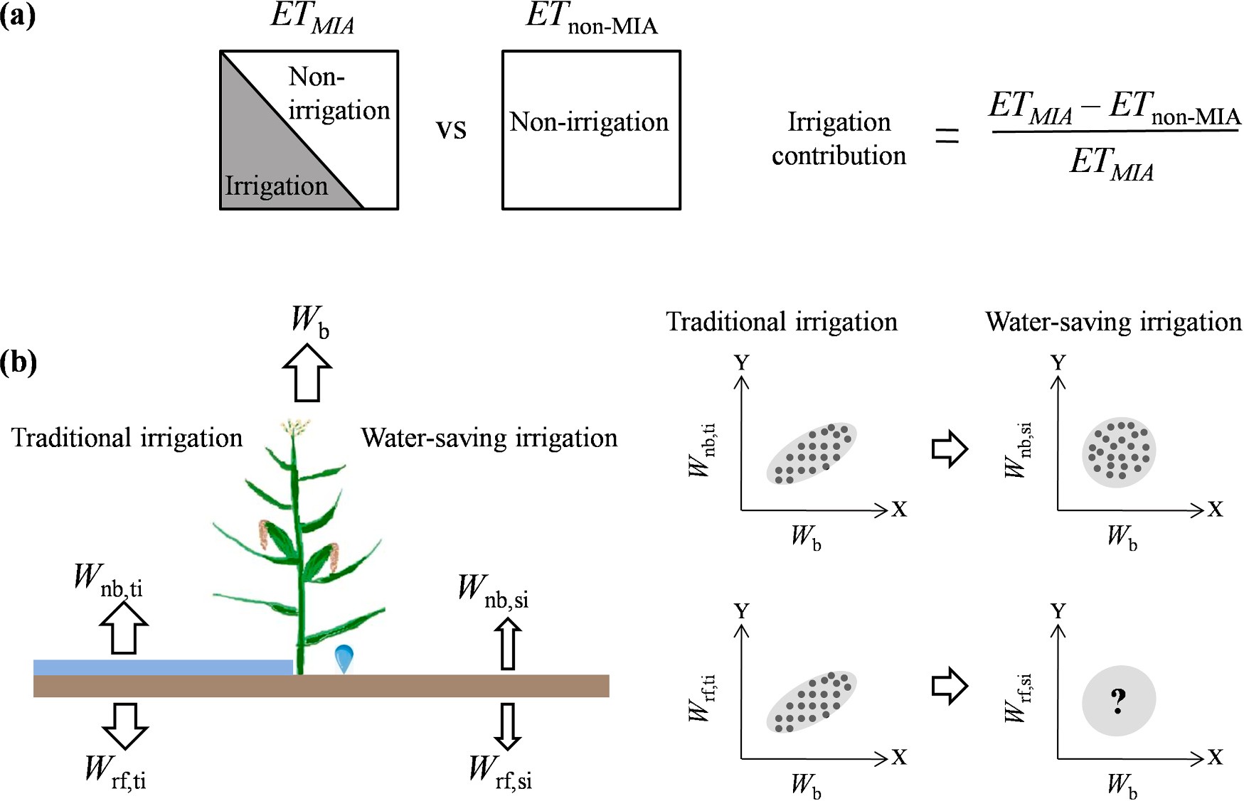
Fig. 2. (a) Estimation of irrigation contribution in satellite-based gridded ET in Major Irrigation Area (MIA). (b) Explanation of water-savings theory. In traditional flooding irrigation, there is linear relationship between beneficial water consumption (Wb) and non-beneficial water consumption (Wnb) or return flow (Wrf). While in water-saving irrigation, there is much weaker relationship between Wb and Wnb and the relationship between Wb and Wrf needs to be investigated.

irrigation water use. Meanwhile, soil evaporation and return flow are increasing at the same time because water is evenly applied to crop and soil. Therefore it is reasonable to assume that under traditional flooding irrigation, crop transpiration (beneficial water consumption, Wb) is positively and linearly related to soil evaporation (non-beneficial water consumption, Wnb) and return flow (Wrf) (Fig. 2b).

Under water-saving irrigation, however, the relationship between crop transpiration and soil evaporation/return flow is probably different with that under traditional flooding irrigation. On one hand, the cor- relation between crop transpiration and soil evaporation (hereafter called Wb-Wnb relationship) would be much weaker. On the other hand, the linear relationship between crop transpiration and return flow (hereafter called Wb-Wrf relationship) is largely uncertain and waiting for investigation. This is because (1) some water-saving technologies mainly work on reducing soil evaporation rather than return flow, e.g., soil mulching. Lots of literatures documented that soil mulching is the most widely used water-saving technologies in some regions such as China and India (Qin et al., 2015; Sun et al., 2020). Other water-saving technologies can reduce soil evaporation and return flow simulta- neously, e.g., sprinkler and drip irrigation, but their application is quite limited due to high capital investment (Polak et al., 1997). (2) Water is also heavily percolated in the process of transportation from river to the

field. It is reported that canals waste up 30–50% of total volume of water

transported according to different locations and management (Mohammadi et al., 2019). Additionally, improper management, such as more irrigation times, inadequate maintenance and emitter clogging, can greatly lower on-farm efficiency of sprinkler and drip irrigation (Levidow et al., 2014).

Therefore, by comparison of different Wb-Wnb relationship under two irrigation modes, the water savings from reducing soil evaporation can be estimated. We further investigate the new Wb-Wrf relationship under water-saving irrigation and estimate the water savings from the change of return flow accordingly.

2.2.3. Estimation of area-induced changes in irrigation water use

Two scenarios, irrigated lands varied (Svary) and irrigated lands fixed (Sfix) were designed to explore the irrigation change induced by area change. In Svary, irrigated lands changed every five years according to HID datasets (1980 irrigated lands used for estimating irrigation in

1980–1984 and 1985 for 1985–1989, 1990 for 1990–1994, 1995 for

1995–1999, 2000 for 2000–2004 and 2005 for 2005 to the end of study

period). In Sfix, 1980 irrigated lands were used to estimate irrigation in all years. Thus, the area-induced irrigation change (Ca) was calculated as:

Ca = (WSvary,2010s-WSfix,2010s) / (WSvary,2010s-WSvary,1980s) * 100% (6)

where WSvary,2010s and WSfix,2010s represent water flows (withdrawal, consumption or return flow) averaged for the 2010s (2010–2018) under Svary and Sfix scenarios respectively, WSvary,1980s represents the water flows averaged for the 1980s (1980–1989) under Svary scenario.

2.2.4. Calculation of water savings at field and regional scale

To calculate water savings, firstly, water consumption was divided into beneficial (essentially transpiration) and non-beneficial (essentially soil evaporation) water consumption. Canopy interception was excluded because satellite-based canopy interception is obtained from only pre- cipitation, rather than overhead irrigation. We further assumed that

5–25% of return flow was percolated into saline aquifers thus can be

seen as loss/non-recoverable. The lower boundary was determined by the proportion of land salinized due to irrigation (FAO, 2010) and the upper boundary was defined by a latest global dataset of groundwater salinity measurements (Thorslund and van Vliet, 2020). According to this dataset, globally approximate 75% of groundwater in Major Irri- gation Areas (MIA) was considered suitable for irrigation as the

measured electrical conductivity is less than 2500 μS/cm (https://mrccc

.org.au/wp-content/uploads/2013/10/Water-Quality-Salinity-Stan dards.pdf).

Secondly, it was necessary to differentiate water savings at field scale from that at region scale. Water-savings at field scale was defined as the

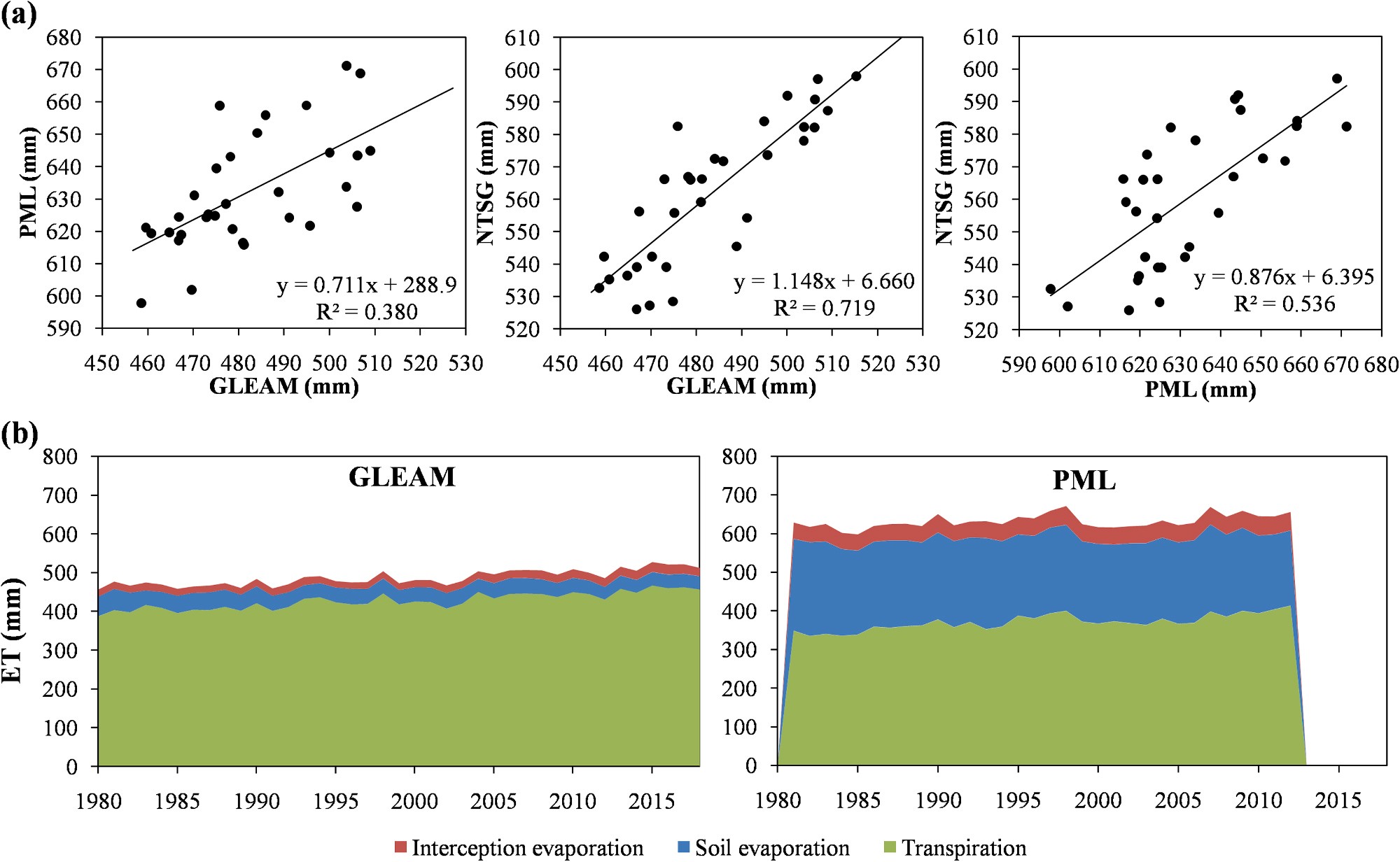
Fig. 3. Global comparison of three satellite-based ET partitions and their components — interception evaporation, soil evaporation and transpiration.

sum of saved water from non-beneficial water consumption and all re- turn flow. While water-savings at region scale was defined as the sum of saved water from non-beneficial water consumption and non- recoverable return flow percolating to saline aquifers.

Savingfield = Σ∆Wnb + Σ∆Wrf =Σ(Wnb,ti - Wnb,si) +Σ(Wrf,ti - Wrf,si) (7)

Savingregion = Σ∆Wnb + a*Σ∆Wrf =Σ(Wnb,ti - Wnb,si) + a*Σ(Wrf,ti - Wrf,si)(8)

where Savingfield and Savingregion are the accumulated 40-years water- savings from the 1980s to 2010s at field and region scales respec- tively; Wnb,si and Wrf,si are non-beneficial water consumption and return flow from water-saving irrigation; Wnb,ti and Wrf,ti are non-beneficial water consumption and return flow from traditional flooding irriga- tion; ∆Wnb is the difference between Wnb,ti and Wnb,si; and ∆Wrf is the difference between Wrf,ti and Wrf,si, a denotes the proportion of saline groundwater which is not suitable for irrigation. The range of a is set to

5–25%.

Based on the water-saving theory and following analysis, the irri- gation mode in newly-developed irrigated lands (Svary-Sfix scenario) was considered as traditional and that in old irrigated lands (Sfix scenario) was seen as water-saving. Therefore, the Wb-Wnb and Wb-Wrf relation- ships under traditional flooding irrigation mode were compared with those under water-saving irrigation mode to estimate water savings.

3. Results

3.1. Comparison of three partitioned satellite-based ET products

Fig. 3a shows that the three satellite-based ET partitions agree fairly well at global scale, with high correlation coefficients of 0.62 (GLEAM vs PML), 0.73 (PML vs NTSG) and 0.85 (GLEAM vs NTSG), respectively. On average, PML has the highest global average ET, GLEAM has the lowest global average ET and NTSG is in the middle. Furthermore, GLEAM and PML could be involved in comparison of ET components (the

components of NTSG are unavailable). In spite of the high correlation in total ET between the two datasets, large differences exist in their three

components — transpiration, soil evaporation and canopy interception.

The biggest inconsistency could be seen for soil evaporation, comprising 8% (GLEAM) and 34% (PML) of total ET respectively (Fig. 3b). This is probably caused by the different algorithms used for soil moisture constraints in GLEAM and PML models.

3.2. Global and regional changes in irrigation water flows for the past 40 years

Global and regional water withdrawal, water consumption and re- turn flow estimated from three satellite-based ET partitions show

notable differences for the period 1980–2000s due to the inconsistency

in ET components (Fig. 4). At global scale, PML has the higher estimates of irrigation water flows, with around 1500 km3 yr—1 for water with- drawal, 700 km3 yr—1 for water consumption and 800 km3 yr—1 for re- turn flow. GLEAM has the lower estimates, with about 1100 km3 yr—1 for water withdrawal, 400 km3 yr—1 for water consumption and 700 km3 yr—1 for return flow. Water consumption of NTSG is the highest with about 720 km3 yr—1. At four hot-spot irrigation areas, GLEAM has higher

estimates of water withdrawal and return flow than PML in Western US

and North China Plain, and NTSG has the highest estimates of water consumption in Western US and Central Asia. It should be noted that in Western US and Northwest India. there are large discrepancies in esti- mates of irrigation water flows among different ET datasets, but the uncertainties are largely reduced in North China Plain and Central Asia. This might be attributed to the difficulties in ET estimation in complex terrains.

Fig. 4 also shows that in comparison with Sfix scenario, the increase of irrigation water flows in the period 1980–2010s is largely caused by

newly-developed irrigated lands. Globally, this area-induced increase in water withdrawal accounts for 49% (GLEAM) and 82% (PML) of total increase, while for water consumption the increase is 56% (GLEAM),

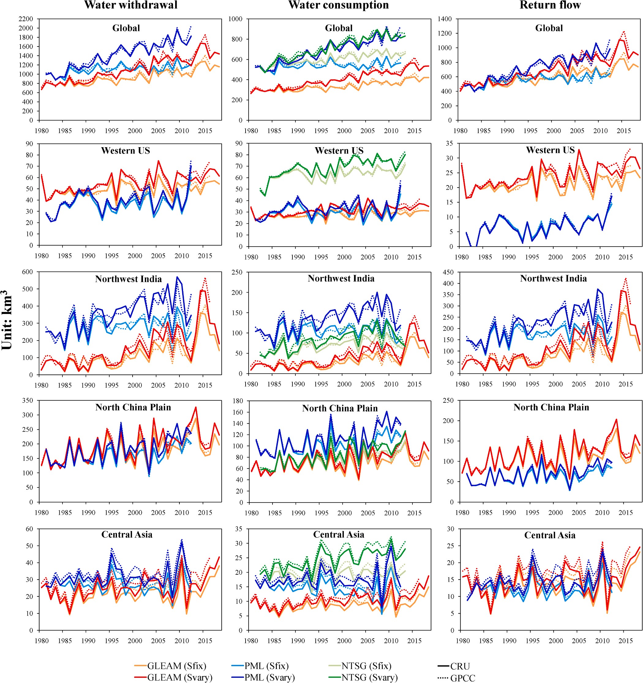
Fig. 4. Estimated water withdrawal, water consumption and return flow from the 1980s to the 2010s based on three satellite-based ET partitions at globe and four hot-spot irrigated areas. Description of the satellite-based ET products — GLEAM, PML and NTSG and of the two precipitation products — CRU and GPCC is given in Table 1. Svary corresponds to flows calculated for varied irrigated lands throughout the four decades and Sfix for fixed irrigated lands in 1980s.

94% (PML) and 71% (NTSG) of the total increase. Also the area-induced increase in return flow accounts for 46% (GLEAM) and 74% (PML) of the total increase. Regionally, over 30% of increase in irrigation water flows in North China Plain is induced by area increase, with 34% (GLEAM) and 43% (PML) for water withdrawal, 40% (GLEAM), 52% (PML), and 35% (NTSG) for water consumption, and 31% (GLEAM) and 43% (PML) for return flow. For Central Asia, this area-induced increase in water withdrawal is 47% (GLEAM) and 77% (PML), while 61% (GLEAM), 100% (PML) and 111% (NTSG) for water consumption, and 33%

(GLEAM) and 54% (PML) for return flow. In Western US and Northwest India, the area-induced increase in irrigation water flows shows large discrepancies in estimates from different ET datasets, with 62% (GLEAM) vs 37% (PML) in Western US and 35% (GLEAM) vs 97% (PML)

in Northwest India for water withdrawal, 63% (GLEAM), 54% (PML) vs 59% (NTSG) in Western US and 36% (GLEAM), 145% (PML) vs 64%

(NTSG) in Northwest India for water consumption, 61% (GLEAM) vs 18% (PML) in Western US and 34% (GLEAM) vs 83% (PML) in North- west India for return flow.

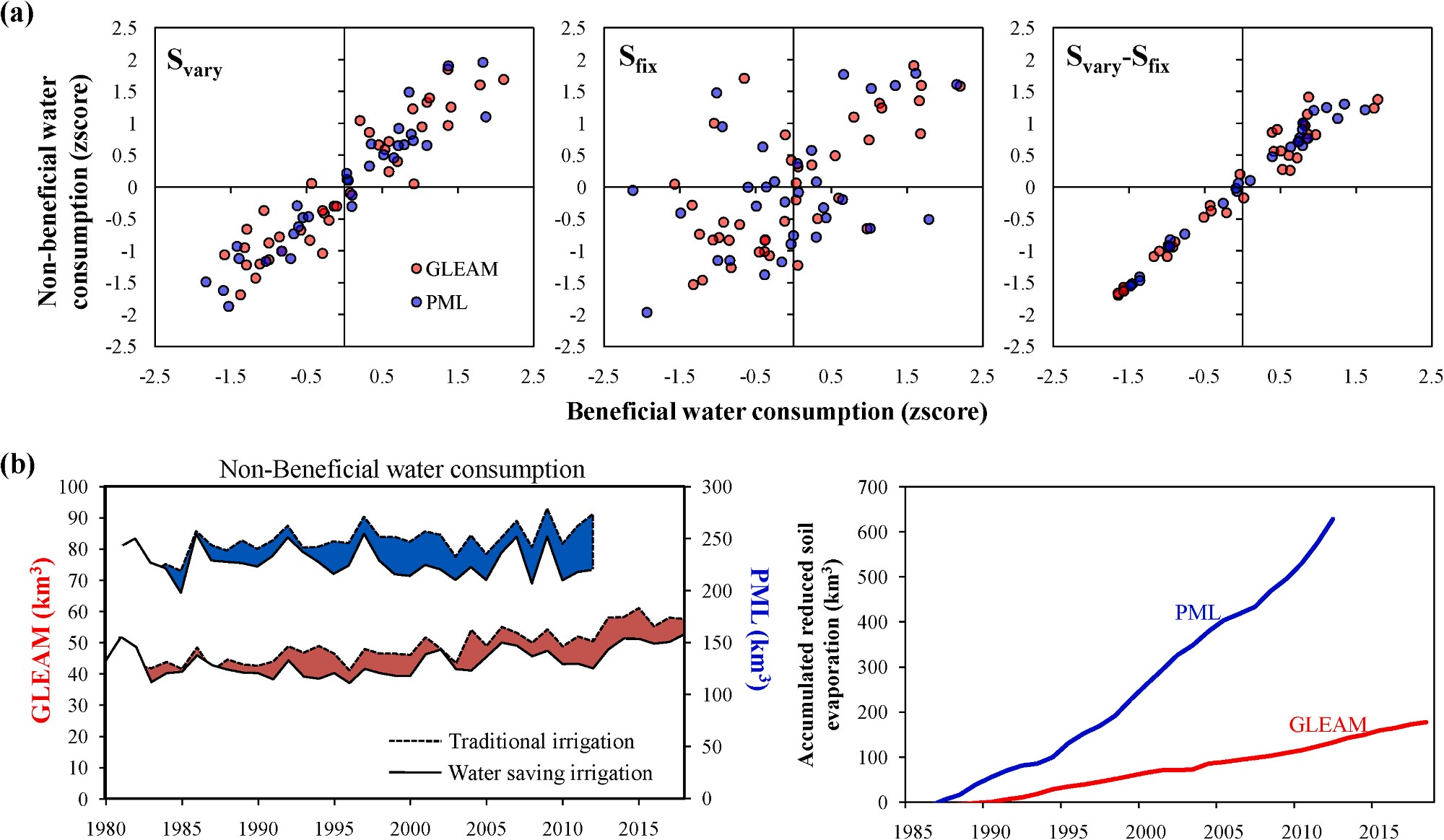
Fig. 5. (a) Comparison of beneficial and non-beneficial water consumptions for all (Svary), old (Sfix) and newly-developed (Svary-Sfix) irrigated lands and (b) the difference of non-beneficial water consumption under two irrigation modes and the accumulated saved water from the reduction of soil evaporation in the period of the 1980s to the 2010s across the globe. zscore denotes the standard scores of beneficial and non-beneficial water consumptions which have been normalized by subtracting the mean then dividing the standard deviation.

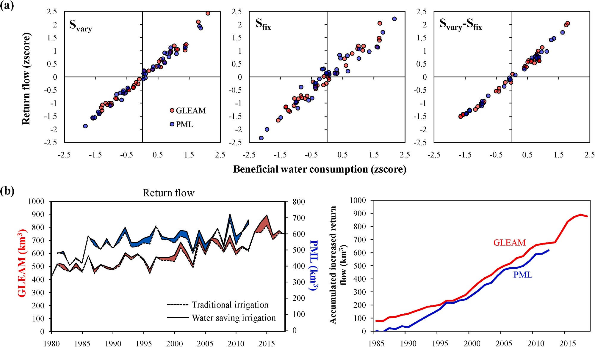
Fig. 6. (a) Comparison of beneficial water consumption and return flow for all (Svary), old (Sfix) and newly-developed (Svary-Sfix) irrigated lands and (b) the difference of return flow under two irrigation modes and the accumulated increase in return flow from the 1980s to the 2010s across the globe. zscore denotes the standard scores of beneficial water consumptions and return flow which have been normalized by subtracting the mean then dividing the standard deviation.

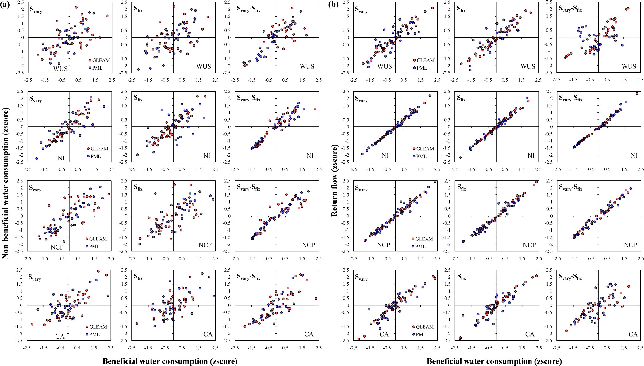
Fig. 7. Comparison of Wb-Wnb and Wb-Wrf relationships for all (Svary), old (Sfix) and newly-developed (Svary-Sfix) irrigated lands in four hot-spot irrigated areas for the past 40 years (1980s–2010s). WUS is Western United States, NI is Northwest India, NCP is North China Plain and CA is Central Asia. zscore denotes the standard scores of irrigation water flows which have been normalized by subtracting the mean then dividing the standard deviation.

3.3. Global Wb-Wnb and Wb-Wrf relationships under two irrigation modes

Fig. 5a shows the relationships between beneficial and non- beneficial (Wb-Wnb relationship) water consumption in three scenarios with different irrigated lands (Svary, Sfix and Svary-Sfix). There is strong

and positive Wb-Wnb relationship (R2 = 0.86 for GLEAM and R2 = 0.91

for PML) in Svary scenario while the correlation becomes much weaker (R2 0.46 for GLEAM and R2 0.21 for PML) in Sfix scenario. This

finding clearly implies that water-saving technologies are mainly applied in old irrigated lands (Sfix) and effectively reduce soil evapora- tion, while those newly-developed irrigated lands (Svary-Sfix) are still

dominant by traditional flooding irrigation (R2 = 0.95 for GLEAM and

R2 = 0.98 for PML). Therefore the irrigated lands of Sfix scenario is seen

as water-saving while those of Svary-Sfix scenario can be seen as tradi-

tional. By comparison the Wb-Wnb relationship of Svary-Sfix scenario with that of Sfix scenario, it is estimated that totally ~ 178 km3 (GLEAM) or

629 km3 (PML) water is saved during the past 40 years through reducing soil evaporation in old irrigated lands (Fig. 5b).

Fig. 6a shows the relationships between beneficial water consump-

tion and return flow (Wb-Wrf correlation) in three scenarios with different irrigated lands (Svary, Sfix and Svary-Sfix). Similarly, strong and positive Wb-Wrf relationship is noted in Svary scenario (R2 0.98 for

GLEAM and R2 0.99 for PML). However, the Wb-Wrf relationship is

also strong in Sfix scenario (R2 0.97 for GLEAM and R2 0.93 for PML) and Svary-Sfix scenario (R2 0.98 for GLEAM and R2 0.99 for PML). It

implies the inefficiency in reducing return flow of water-saving tech- nologies. Contrary to general expectations, it is found that more return flow in irrigated lands where water-saving technologies are applied

when compare the Wb-Wrf relationship of Svary-Sfix scenario with that of Sfix scenario. This might be caused by the increase of cropping intensity and the replacement of original crops by water-intensive crops, which bring more irrigation water demand and in turn more percolation. It is

estimated that water savings from the change of return flow is 877 km3 (GLEAM) or 618 km3 (PML), implying that global return flow has increased during the 40 years in old irrigated lands in spite of

wide application of water-saving technologies (Fig. 6b).

3.4. Regional Wb-Wnb and Wb-Wrf relationships under two irrigation modes

At the four hot-spot irrigated areas, the water-saving effect is different (Fig. 7). In Western US, the relative weak Wb-Wnb relationships

(R2 0.37 for GLEAM and R2 0.64 for PML in Svary scenario, R2 0.27 for GLEAM and R2 0.56 for PML in Sfix scenario and R2 0.55 for GLEAM and R2 0.8 for PML in Svary-Sfix scenario) show that water-

saving technologies are widely used in all irrigation lands. Also the Wb-Wrf relationships are weaker in Western US than other three regions (R2 0.96 for GLEAM and R2 0.7 for PML in Svary and Sfix scenarios

while R2 0.82 for GLEAM and R2 0.22 for PML in Svary-Sfix scenario).

In Northwest India, the strong Wb-Wnb relationships (R2 0.92 for GLEAM and R2 0.7 for PML in Svary scenario, R2 0.89 for GLEAM and R2 0.42 for PML in Sfix scenario and R2 0.88 for GLEAM and R2

0.93 for PML in Svary-Sfix scenario) and Wb-Wrf relationships (R2

0.99 for all products and scenarios) in all scenarios show that the application of water-saving technologies are limited in this region. In

North China Plain, the relatively weak Wb-Wnb relationships (R2 = 0.49

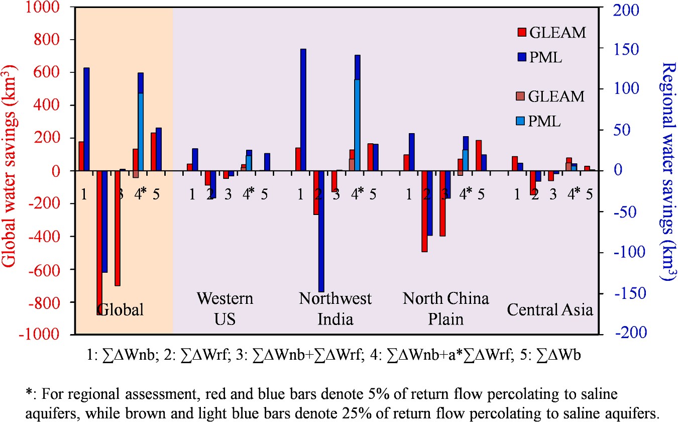Fig. 8. Water savings at field and region scale across the

globe and in four hot-spot irrigated areas during the period of 1980–2010s. The y-axis in the left denotes the global water savings while the y-axis in the right denotes the regional water savings. Σ∆Wnb represents accumulated

water savings from the reduction of soil evaporation, Σ∆Wrf

represents accumulated water savings from the change of return flow, Σ∆Wnb+Σ∆Wrf is total water savings at field scale, Σ∆Wnb+a*Σ∆Wrf is total water savings at regional scale, ΣWb is accumulated increased beneficial water con-

sumption from the increase of crop transpiration in past 40 years. For regional water-saving assessment, red and blue bars denote 5% of return flow percolating to saline aqui- fers, while brown and light blue bars denote 25% of return flow percolating to saline aquifers (For interpretation of the references to color in this figure legend, the reader is referred to the web version of this article).

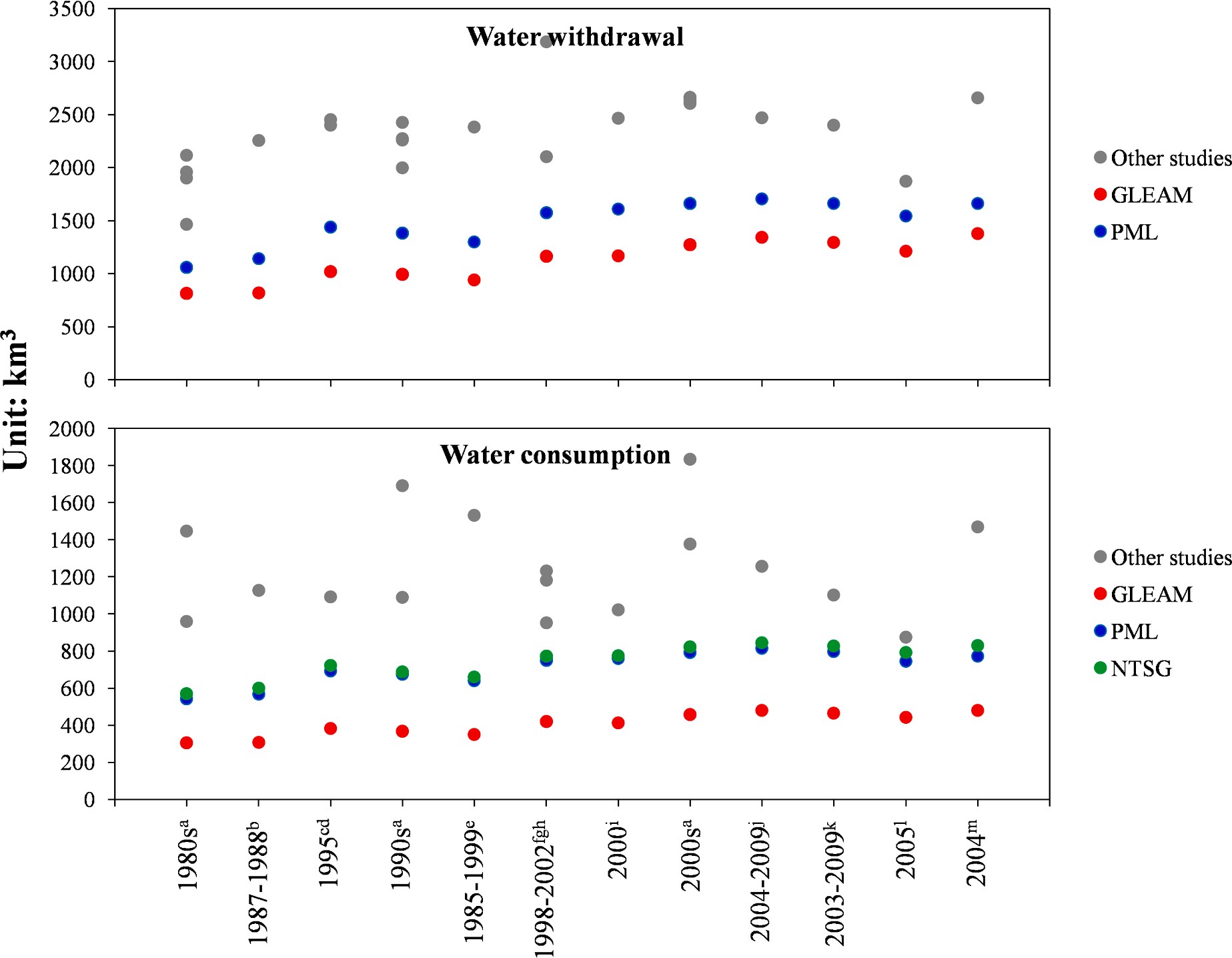
Fig. 9. Comparison of estimates of irrigation water consumption and water withdrawal between this study and other studies. (a) Wada et al. (2011); (b) Hanasaki et al. (2006); (c) Oki et al. (2001); (d) Dӧll and Siebert (2002); (e): Hanasaki et al. (2010); (f) Siebert and Dӧll (2010); (g) Dӧll et al. (2012); (h) Liu and Yang (2010);

(i) Pokhrel et al. (2012); (j) Jӓgermeyr et al. (2015); (k) Dӧll et al. (2014); (l) Chen et al. (2019); and (m) Hoogeveen et al. (2015).

for GLEAM and R2 = 0.87 for PML in Svary scenario, R2 = 0.32 for GLEAM and R2 = 0.8 for PML in Sfix scenario and R2 = 0.81 for GLEAM and R2 = 0.98 for PML in Svary-Sfix scenario) and relative strong Wb-Wrf relationships (R2 = 0.99 for GLEAM and R2 = 0.95 for PML in Svary and Sfix scenario, and R2 = 0.98 for GLEAM and R2 = 0.97 for PML in Svary-

Sfix scenario) implies that traditional flooding irrigation is dominant here but soil evaporation is effectively reduced by other methods such as

straw mulching (Qin et al., 2015). In Central Asia, water-saving tech- nologies might be partly used because of relative weak Wb-Wnb re- lationships (R2 0.61 for GLEAM and R2 0.51 for PML in Svary

scenario, R2 0.6 for GLEAM and R2 0.47 for PML in Sfix scenario and

R2 0.69 for GLEAM and R2 0.71 for PML in Svary-Sfix scenario) and Wb-Wrf relationships (R2 0.95 for GLEAM and R2 0.82 for PML in Svary scenario, R2 0.98 for GLEAM and R2 0.79 for PML in Sfix sce- nario and R2 0.71 for GLEAM and R2 0.65 for PML in Svary-Sfix

scenario).

3.5. Water-savings assessment at field and regional scale

Given that water-saving technologies are mainly applied on old irrigated lands, water savings are estimated only in old irrigated lands across the globe and the four hot-spot irrigated areas (Fig. 8). In spite of large difference between GLEAM and PML estimates, results show high consistency in water savings assessment. At both globe and four hot-spot irrigated areas, water savings from non-beneficial water consumption are positive, implying that water-saving technologies reduce soil evap- oration. Conversely, water savings from return flow is negative, implying increasing return flow despite water-saving technologies are widely used. As a result, water savings is negative at field scale because the accumulated increased return flow is more than the accumulated reduced non-beneficial water consumption. It means that water-saving technologies fail to save water at field scale as all return flow is considered as loss. However, if most return flow percolating into fresh aquifers is seen as beneficial, water savings become positive over globe and four hot-spot irrigated areas, which means that water-saving tech- nologies do save water at regional scale. Meanwhile, accumulated increased beneficial water consumption (crop transpiration) exceeds the water savings at regional scale in the four decades. This explains the paradox between wide application of water-saving technologies and more severe regional water shortage over globe.

In spite of more return flow in irrigated lands, it does not mean the

recovery of water table. This is because (1) more irrigation water is needed from newly-developed irrigated lands and the increasing bene- ficial water consumption; (2) Irrigation water was probably from deep aquifer withdrawal, but it recharged to shallow aquifers and caused higher depletion rate in deep aquifers (Feng et al., 2013).

4. Discussions

4.1. Satellite-based method reliability and uncertainty

Previous studies using agro-hydrological models report that irriga- tion water consumption ranging from 800 to 1600 km3 yr—1 and water withdrawal from 1500 to 3000 km3 yr—1 (Fig. 9). Moreover on global

scale, irrigation water consumption accounts for ~ 50% of water with- drawal (Gleeson, 2017), which fits the values found by this study. Although our study has lower estimates compared to other studies, we think the biases are acceptable because (1) our estimation is only con- ducted in cells where more than 20% of area is equipped with irrigation, and (2) some small irrigated areas are ignored due to the coarse spatial resolution. Among the three products, PML and NTSG estimates are the

highest while GLEAM estimates are the lowest.

In spite of the reasonable global estimation, however, large un- certainties exist for some regions such as Western United States and Northwest India. Besides the influence of complex terrains mentioned above, two other factors are considered attributed to the uncertainties. One is the algorithm of the satellite-based ET partitions. In PML, the soil

evaporation fraction f = min(P/Eeq,1) is used, where P is accumulated

precipitation and Eeq soil equilibrium evaporation (Zhang et al., 2010a,

2010b). This soil moisture availability model works well at daily scale and in Mediterranean type drylands where available soil moisture continually supports ET in a few days after precipitation events. At annual scale, however, PML excessively overestimates soil evaporation because P generally equals ET and thereby makes f approaches 1, especially in drylands. On the other hand, GLEAM likely underestimates soil evaporation because satellites only observe surface soil moisture, which rapidly goes dry in the first stage. The second stage evaporation from capillary flow from deep soil moisture sources is neglected by satellite soil moisture (Lehmann et al., 2018). Another is the rice farming in Northwest India. Rice is the major crop in northern sub-Himalayan

region, which contributes some 15% to India’s entire rice production

(Sharma et al., 2018). In rice system, water is needed in land preparation stage. Then ponding technique is adopted to keep soil saturated during the entire growth period, except for the last 15 days (Chapagain and Hoekstra, 2010). It is not clear how satellite deals with soil evaporation in rice fields as free water evaporation or normal evaporation in arable

lands. However, it probably underestimates soil evaporation at the initial stage of rice growth. Moreover, high variations of 50–85% percolation due to climate, management, soil texture induce large un-

certainties in return flow estimation (Mandal et al., 2019). In recent decades, the changes of cropping pattern from rice to other crops (mainly wheat) in this region leads to more uncertainties of return flow estimation (Bajpai and Volavka, 2005; Ramadas et al., 2019). It is rec- ommended to improve the algorithms of satellite-based ET and the transformation of cropping pattern should be considered in the future.

4.2. Higher water use efficiency towards more water savings and food security

It is reported that water use efficiency for global irrigated lands has significantly increased from 1.52 in 2000 to 1.73 kg/m3 in 2014 (Xue et al., 2015; Ai et al., 2020). Meanwhile, global cereal production has

increased from 2.05 to 2.82 billion tons per year in the same period

(World Bank, 2018). Given that irrigated agriculture produces about 40% of the world’s food (FAO, 2002), it is estimated ~ 21% of increase in irrigation water use from 2000 to 2014. Meanwhile, our results show

only ~ 15% of increase in water withdrawal/consumption, implying that other factors also contribute to the water savings, e.g., the increase of water use efficiency from cultivar change, fertilizer input, better management. Therefore actual water savings would be higher than our estimates if water use efficiency is considered.

Moreover, this study shows that globally area-induced increase ac- counts for over 50% of total increase in irrigation water flows from 1980s to 2000s, which implies that ~ 20% of increase in cereal pro- duction is from newly-developed irrigated lands. Unfortunately, the potentials for future increase of cropland expansion is quite limited due to urban encroachment, land degradation, climate change, geographic constraints, and the threat of biodiversity loss (Zabel et al., 2019). Thus it is recommended that the improvement of water use efficiency would be a better solutions for both water and food insecurity in the future.

5. Conclusions

To explore the paradox in irrigation efficiency on global scale, this study estimated global water withdrawal, consumption and return flow from irrigated agriculture for the past 40 years using satellite-based ET partitions. For the first time, the effects of water-saving technologies were quantified across the globe at both field and region scales based on water accounting framework. The results showed that global irrigation water flows kept increasing from the 1980s to the 2010s, with over 50% of the increase due to newly-developed irrigated lands. Water-saving technologies were mainly applied in old irrigated lands, while tradi- tional flooding irrigation was still dominant in newly-developed irri- gated lands. Water-saving technologies effectively reduced soil evaporation, but increasing return flow was found in spite of the wide application of these technologies. At field scale, water-saving technol- ogies failed to save water because the accumulated increased return flow was more than the accumulated decreased non-beneficial water con- sumption (soil evaporation). At regional scale, however, water was saved as the return flow percolated to fresh aquifers was seen as bene- ficial rather than loss. At the same time, accumulated increased bene- ficial water consumption (crop transpiration) exceeded the regional water savings, which explains the paradox between wide application of water-saving technologies and more severe regional water shortage. In the future, more work was required, including exploration of the mechanisms for partitioning satellite-based transpiration and evapora- tion, improvement of gridded irrigation efficiency based on crop type and irrigation system, and the inclusion of water use efficiency.

Financial support

This study was supported by the Strategic Priority Research Program, Chinese Academy of Sciences (Grant no. XDA2004030203), the

International Collaborative Project of the Ministry of Science and Technology of China (Grant no. 2018YFE0110100), the open fund of Key Laboratory of Water Cycle and Related Land Surface Processes, Chinese Academy of Sciences, Institute of Geographic Sciences and Natural Resources Research, Chinese Academy of Sciences (Grant no. WL2019004), the fund of Key Laboratory of Agricultural Water Re- sources, Chinese Academy of Sciences (Study on Global Changes in Agricultural Use/Supply and its impacts on Food Security) and National Natural Science Foundation of China, China (Grant no. 41971262).

Author contributions

XZ did the analyzes, created the figures and wrote the main text of the paper. HL did the data proceeding. YZ, ZS and KM laid the paper structure and polished the language. MA, YY and SH commented on the general text.

Declaration of Competing Interest

The authors declare that they have no known competing financial interests or personal relationships that could have appeared to influence the work reported in this paper.

Data Availability

Global gridded data used in this study are openly available as indi- cated in Section 2.1.

Acknowledgments

Authors sincerely thank Jonas Jӓgermeyr and Dieter Gerten for sharing with us their results on Beneficial Irrigation Efficiency.

Appendix A. Satellite-based ET partitioning algorithms — brief description

Here, we briefly describe the algorithms of the three partitioned satellite-based ET products used in this study — GLEAM, PML and NTSG.

A1 GLEAM

First, the Priestley-Taylor (1972) equation is used to calculate potential evapotranspiration rate Ep (mm day—1) as:

λEp = α Δ (Rn — G) (A1)

where λ (MJ kg—1) is latent heat of vaporization; ∆ (kPa K—1) is slope of saturated vapor pressure curve; γ (kPa K—1) is psychrometric constant; and α is Priestley-Taylor coefficient. In GLEAM, α 0.97 is used to parameterize tall vegetation, while α 1.26 is used in both short vegetation and bare soil (Martens et al., 2017).

Then a semi-empirical stress factor S is used to separate potential evapotranspiration into transpiration and soil evaporation based on water content of vegetation and root zone. The former is related to microwave vegetation optical depth and the latter is calculated using a multi-layer soil model driven by precipitation and microwave surface soil moisture.

ET = Ep × S + Ei, (A2)

where Ei (mm day-1) is interception loss based on refined Gash analytical model (Miralles et al., 2010).

A2 PML

The PML model separates ET into transpiration and soil evaporation as a function of four meteorological variables (precipitation, net radiation, water vapor deficit and aerodynamic conductance) and a biophysical variable (surface conductance) (Zhang et al., 2010a, 2010b, 2017).

λE = εA + .ρcp/γ)DaGa = εAc + .ρcp/γ)DaGa + f εAs

(A3)

ε + 1 + Ga/Gs ε + 1 + Ga/Gc ε + 1

where ε = s/γ, in which γ is psychrometric constant (kPa ℃—1) and s = de* /dTair is slope of the curve relating saturation water vapor pressure to air

temperature; A is available energy absorbed by the surface (MJ m—2 d—1); ρ is density of air (g m—3); cp is specific heat of air at constant pressure (J g—1

℃—1), Da e* -ea is water vapor pressure deficit of air (kPa) between saturation water vapor pressure e* and actual water vapor pressure ea; Ga is aerodynamic conductance (m s—1); Gs is surface conductance; Ac is available energy absorbed by canopy (MJ m—2 d—1); As is available energy absorbed by soil (MJ m—2 d—1); Gc is canopy conductance to water vapor (m s—1); and f is soil evaporation coefficient limited by water.

Gs is expressed as:

Gs = Gc⎢⎣

τ[ ]

⎥⎦ (A4)

where τ = exp(-kALai), kA is extinction coefficient for available energy; Lai is leaf area index; and Gi is "climatological" conductance.

A3 NTSG

NTSG also uses the Penman-Monteith approach to estimate ET.

λE ΔACanopy + ρCp esat — e ga Δ + γ(1 + ga/gs)

λE RH(VPD/k) ΔASoil + ρCp VPDga

Δ + γ × ga/gtotc

(A5)

(A6)

where λ is latent heat of vaporization (J kg—1); A is available energy components for canopy (Acanopy, W m—2) and soil surface (Asoil, W m—2); ∆ d (esat)/dT is slope of curve relating saturated water vapor pressure esat to air temperature T (Pa K—1); esat-e is vapor pressure deficit (VPD, Pa); ρ is air density (kg m—3); Cp is specific heat capacity of air (J kg—1 K—1); γ is psychrometric constant (kPa ℃—1); ga is aerodynamic conductance (m s—1); gs is surface conductance (m s—1); RH (VPD/k) is moisture constraint on soil evaporation; k is parameter to reflect relative sensitivity to VPD; and gtotc is corrected value of total aerodynamic conductance gtot (m s—1).

Here, surface conductance gs is defined by the NDVI-based Jarvis-Stewart formula as:

gs = g0.NDVI)⋅m.Tday)⋅m.VPD) (A7)

where g0(NDVI) is biome-dependent potential value of gs; m(Tday) is temperature stress factor and function of daylight average air temperature Tday; and m(VPD) is water/moisture stress factor and function of VPD.

Appendix B. The validation of HID dataset by the comparison with GFSAD

To verify the reliability of HID dataset, the extent of HID 2005 dataset was compared with that of GFSAD dataset, a 1-km-resolution Crop Dominance product in differentiating irrigated areas from rainfed areas for year 2010 (Thenkabail et al., 2012). The 1-km GFSAD was resampled into 8-km product, complying with the HID resolution and was noted that the extent of the two datasets was most comparable when the proportion of HID AEI was larger than 20% (77620 vs 73230 grids) (Fig. B1). This further approved the definition that MIA was the cells with proportion of HID AEI

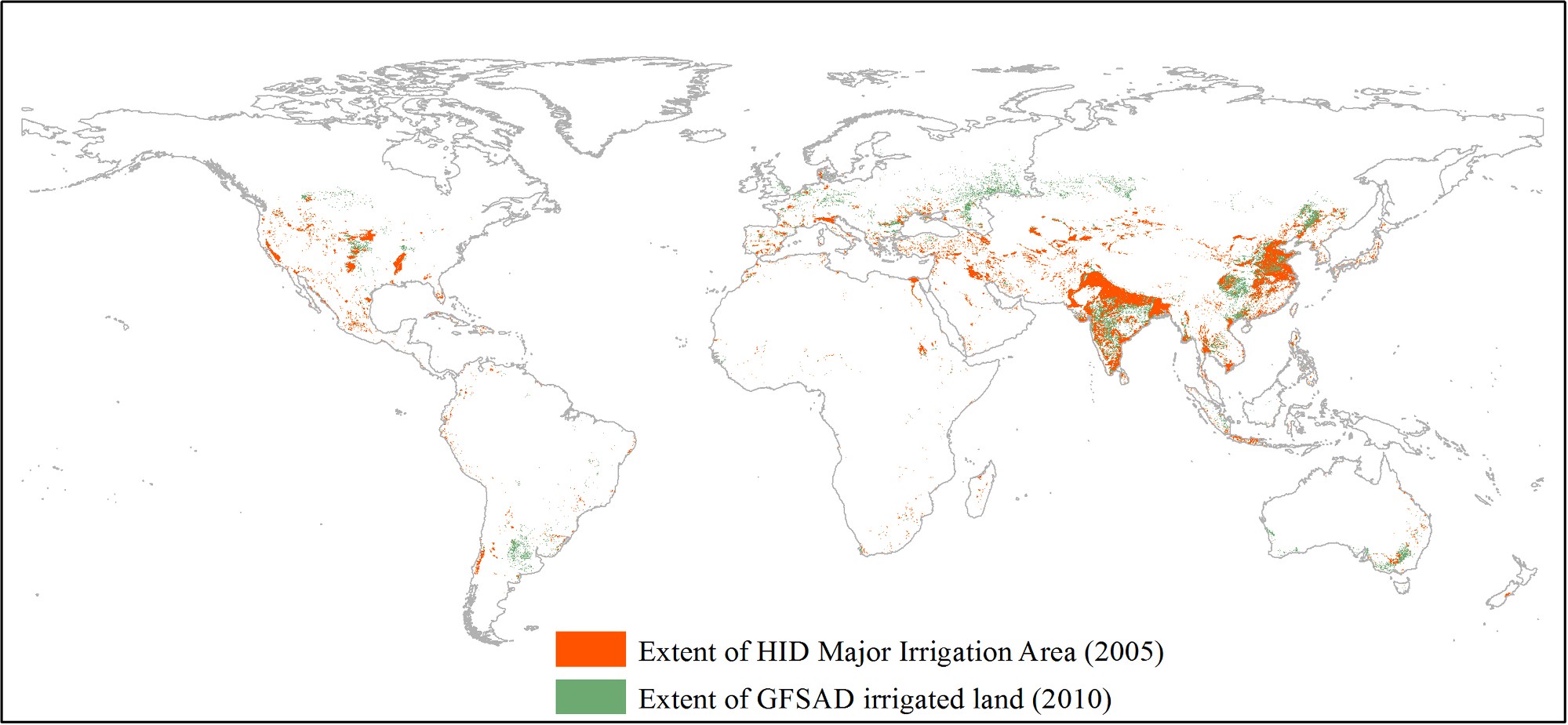
Fig. B1. Comparison of the extent between HID MIA in 2005 and GFSAD irrigated land in 2010.

larger than 20%. The main crops are wheat and maize in North China Plains, wheat and rice in North India, wheat and cotton in Central Asia, wheat, soybean, and maize in North America.

References

Ai, Z., Wang, Q., Yang, Y., Manevski, K., Yi, S., Zhao, X., 2020. Variation of gross primary production, evapotranspiration and water use efficiency for global croplands. Agric. For. Meteorol. 287, 107935.

Bajpai, N., Volavka, N., 2005. Agricultural performance in Uttar Pradesh: a historical account. CGSD Working Paper No. 23. https://academiccommons.columbia. edu/doi/10.7916/D8PK0FF9 . (Accessed 23 June 2020).

Batchelor, C., Hoogeveen, J., Faur`es, J.-M., Peiser, L., 2017. Water Accounting and

Auditing - A Sourcebook. Food and Agriculture Organization of the United Nations, Rome, Italy, p. 2017.

Berbel, J., Gutierrez-Marín, C., Expo´sito, A., 2018. Impacts of irrigation efficiency

improvement on water use, water consumption and response to water price at field level. Agric. Water Manag. 203, 423–429.

Brouwer, C., Prins, K., Heibloem, M., 1989. Irrigation water management: irrigation scheduling. Training Manual No.4, FAO. http://www.fao.org/3/t7202e/t7202e00. htm . (Accessed 25 December 2020).

Burt, C.M., Howes, D.J., Mutziger, A., 2001. Evaporation estimates for irrigated agriculture in California. In: Conference Proceedings of the Annual Irrigation Association Meeting. San Antonio, Texas.

Chapagain, A.K., Hoekstra, A.Y., 2010. The green, blue and grey water footprint of rice from both a production and consumption perspective. Value of Water Research Report Series No. 40, UNESCO-IHE Institute, Delft, The Netherlands.

Chen, Y., Feng, X., Fu, B., Shi, W., Yin, L., Lv, Y., 2019. Recent global cropland water

consumption constrained by observations. Water Resour. Res. 55, 3708–3738.

Di, N., Wang, Y., Clothier, B., Liu, Y., Jia, L., Xi, B., Shi, H., 2019. Modeling soil evaporation and the response of the crop coefficient to leaf area index in mature Populus tomentosa planations growing under different soil water availabilities.

Agric. For. Meteorol. 264, 125–137.

Dӧll, P., Siebert, S., 2002. Global modeling of irrigation water requirements. Water

Resour. Res. 38, 8-1–8-10.

Dӧll, P., Hoffmann-Dobev, H., Portmann, F.T., Siebert, S., Eicker, A., Rodell, M., Strassberg, G., Scanlon, B.R., 2012. Impact of water withdrawals from groundwater

and surface water on continental water storage variations. J. Geodyn. 59–60, 143–156.

Dӧll, P., Muller Schmied, H., Schuh, C., Portmann, F.T., Eicker, A., 2014. Global-scale assessment of groundwater depletion and related groundwater abstractions: combining hydrological modeling with information from well observations and

GRACE satellites. Water Resour. Res. 50, 5698–5720.

FAO, 2002. Crops and Drops, Making the Best Use of Water for Agriculture. Food and Agriculture Organization of the United Nations, Rome, Italy (Accessed 25 December 2020). http://www.fao.org/3/Y3918E/y3918e00.htm.

FAO, 2010. Agriculture and water quality interactions: a global overview. SOLAW Background Thematic Report - TR08. http://www.fao.org/3/a-bl092e.pdf . (Accessed 20 December 2020).

Feng, W., Zhong, M., Lemoine, J.-M., Biancale, R., Hsu, H.-T., Xia, J., 2013. Evaluation of groundwater depletion in North China Plain using the Gravity Recovery and Climate Experiment (GRACE) data and ground-based measurements. Water Resour. Res. 49,

2110–2118.

Fishman, R., Devineni, N., Raman, S., 2015. Can improved agricultural water use

efficiency save India’s groundwater? Environ. Res. Lett. 10, 084022.

Gleeson, T., 2017. What is the difference between ’water withdrawal’ and ’water consumption’, and why do we need to know? AGU blogs. https://blogs.agu.org/

waterunderground/2017/06/26/difference-water-withdrawal-water-consu mption-need-know/ . (Accessed 25 December 2020).

Gleick, P.H., Christian-Smith, J., Cooley, H., 2011. Water-use efficiency and productivity: rethinking the basin approach. Water Int. 36 (7), 784–789.

Grafton, R.Q., Williams, J., Perry, C.J., Molle, F., Ringler, C., Steduto, P., Udall, B., Wheeler, S.A., Wang, Y., Garrick, D., Allen, R.G., 2018. The paradox of irrigation

efficiency. Science 361 (6404), 748–750.

Haddeland, I., Skaugen, T., Lettenmaier, D.P., 2006. Anthropogenic impacts on continental surface water fluxes. Geophys. Res. Lett. 33, L08406.

Haddeland, I., Heinke, J., Biemans, H., Eisner, S., Flo¨rke, M., Hanasaki, N.,

Konzmann, M., Ludwig, F., Masaki, Y., Schewe, J., Stacke, T., Tessler, Z.D., Wada, Y., Wisser, D., 2014. Global water resources affected by human interventions and climate change. PNAS 111 (9), 3251–3256.

Hanasaki, N., Kanae, S., Oki, T., 2006. A reservoir operation scheme for global river

routing models. J. Hydrol. 327 (1–2), 22–41.

Hanasaki, N., Inuzuka, T., Kanae, S., Oki, T., 2010. An estimation of global virtual water

flow and sources of water withdrawal for major crops and livestock products using a global hydrological model. J. Hydrol. 384 (3), 232–244.

Hoogeveen, J., Faur`es, J.M., Peiser, L., Burke, J., van de Giesen, N., 2015. GlobWat—a

global water balance model to assess water use in irrigated agriculture. Hydrol. Earth

Syst. Sci. 19 (9), 3829–3844.

Howell, T.A., 1990. Relationships between crop production and transpiration, evapotranspiration, and irrigation. In: Stewart, B.A., Nielson, D.R. (Eds.), Irrigation of Agricultural Crops, Agronomy Monograph, 30. ASA, CSSA and SSSA, Madison, WI, USA., pp. 391–434

J¨agermeyr, J., Gerten, D., Heinke, J., Schaphoff, S., Kummu, M., Lucht, W., 2015. Water

savings potentials of irrigation systems: global simulation of processes and linkages. Hydrol. Earth Syst. Sci. 19, 3073–3091.

Karimi, P., Bastiaanssen, W.G.M., Molden, D., 2013a. Water Accounting Plus (WA ) - a water accounting procedure for complex river basins based on satellite

measurements. Hydrol. Earth Syst. Sci. 17, 2459–2472.

Karimi, P., Bastiaanssen, W.G.M., Molden, D., Cheema, M.J.M., 2013b. Basin-wide water

accounting based on remote sensing data: an application for the Indus Basin. Hydrol. Earth Syst. Sci. 17, 2473–2486.

Kendy, E., Zhang, Y., Liu, C., Wang, J., Steenhuis, T., 2004. Groundwater recharge from

irrigated cropland in the North China Plain: case study of Luancheng County, Hebei Province, 1949-2000. Hydrol. Process. 18, 2289–2302.

Kummu, M., Guillaume, J.H.A., de Moel, H., Eisner, S., Flӧrke, M., Porkka, M., Siebert, S.,

Veldkamp, T.I.E., Ward, P.J., 2016. The world’s road to water scarcity: shortage and stress in the 20th century and pathways towards sustainability. Sci. Rep. 6, 38495.

Lehmann, P., Merlin, O., Gentine, P., Or, D., 2018. Soil texture effects on surface resistance to bare soil evaporation. Geophys. Res. Lett. 45 (19), 10398–10405.

Leuning, R., Zhang, Y., Rajaud, A., Cleugh, H., Kevin, T., 2008. A simple surface conductance model to estimate regional evaporation using MODIS leaf area index and the Penman-Monteith equation. Water Resour. Res. 44, W10419.

Levidow, L., Zaccaria, D., Maia, R., Vivas, E., Todorovic, M., Scardigno, A., 2014. Improving water-efficient irrigation: prospects and difficulties of innovative

practices. Agric. Water Manag. 146, 84–94.

Liao, L., Zhang, L., Bengtsson, L., 2008. Soil moisture variation and water consumption of

spring wheat and their effects on crop yield under drip irrigation. Irrig. Drain. Syst. 33 (3–4), 253–270.

Liu, J., Yang, H., 2010. Spatially explicit assessment of global consumptive water uses in

cropland: green and blue water. J. Hydrol. 384, 187–197.

Mandal, K.G., Thakur, A.K., Ambast, S.K., 2019. Current rice farming, water resources

and micro-irrigation. Curr. Sci. 16 (4), 568–576.

Martens, B., Miralles, D.G., Lievens, H., van der Schalie, R., de Jeu, R.A.M., Fern´andez- Prieto, D., Beck, H.E., Dorigo, W.A., Verhoest, N.E.C., 2017. GLEAM v3: satellite-

based land evaporation and root-zone soil moisture. Geosci. Model Dev. 10, 1903–1925.

Miralles, D.G., Gash, J.H., Holmes, T.R.H., de Jeu, R.A.M., Dolman, A.J., 2010. Global canopy interception from satellite observations. J. Geophys. Res. 115, D16122.

Miralles, D.G., Holmes, T.R.H., De Jeu, R.A.M., Gash, J.H., Meesters, A.G.C.A.,

Dolman, A.J., 2011. Global land-surface evaporation estimated from satellite-based observations. Hydrol. Earth Syst. Sci. 15, 453–469.

Mohammadi, A., Rizi, A.P., Abbasi, N., 2019. Field measurement and analysis of water losses at the main and tertiary levels of irrigation canals: Varamin Irrigation Scheme, Iran. Glob. Ecol. Conserv. 18, e00646.

Molle, F., Tanouti, O., 2017. Squaring the circle: agricultural intensification vs. water conservation in Morocco. Agric. Water Manag. 192, 170–179.

Müller, C., Elliott, J., Kelly, D., Arneth, A., Balkovic, J., Ciais, P., Deryng, D., Folberth, C., Hoek, S., Izaurralde, R.C., Jones, C.D., Khabarov, N., Lawrence, P., Liu, W., Olin, S.,

Pugh, T.A.M., Reddy, A., Rosenzweig, C., Ruane, A.C., Sakurai, G., Schmid, E., Skalsky, R., Wang, X., de Wit, A., Yang, H., 2019. The global gridded crop model intercomparison phase 1 simulation dataset. Sci. Data 6, 50.

Oki, T., Agata, Y., Kanae, S., Saruhashi, T., Yang, D., Musiake, K., 2001. Global assessment of current water resources using total runoff integrating pathways.

Hydrol. Sci. J. 46 (6), 983–995.

Perry, C., Steduto, P., Karajeh, F., 2017. Does Improved Irrigation Technology Save Water? A Review of the Evidence, in Discussion Paper on Irrigation and Sustainable Water Resources Management in the Near East and North Africa. Food and Agriculture Organization of the United Nations, Cairo, Egypt, p. 2017.

Perry, C.J., 2007. Efficient irrigation; inefficient communication; flawed recommendations. Irrig. Drain. 56, 367–378.

Perry, C.J., Steduto, P., Allen, R.G., Burt, C.M., 2009. Increasing productivity in irrigated agriculture: agronomic constraints and hydrological realities. Agric. Water Manag.

96, 1517–1524.

Pokhrel, Y., Hanasaki, N., Koirala, S., Cho, J., Yeh, P.J.F., Kim, H., Kanae, S., Oki, T., 2012. Incorporating anthropogenic water regulation modules into a land surface

model. J. Hydrometeorol. 13 (1), 255–269.

Polak, P., Nanes, B., Adhikari, D., 1997. A low cost drip irrigation system for small

farmers in developing countries. J. Am. Water Resour. Assoc. 33 (1), 119–124.

Priestley, J.H.C., Taylor, J., 1972. On the assessment of surface heat flux and evaporation

using large-scale parameters. Mon. Weather Rev. 100, 81–92.

Qin, W., Hu, C., Oenema, O., 2015. Soil mulching significantly enhances yields and water and nitrogen use efficiencies of maize and wheat: a meta-analysis. Sci. Rep. 5, 16210.

Ramadas, S., Kumar, T.M.K., Singh, G.P., 2019. Wheat production in India: trends and prospects. IntechOpen: Recent Advances in Grain Crops Research. https://www.inte chopen.com/books/recent-advances-in-grain-crops-research/wheat-production-in- india-trends-and-prospects . (Accessed 23 June 2020).

Scott, C.A., Vicun˜a, S., Blanco-Guti´errez, I., Meza, F., Varela-Ortega, C., 2014. Irrigation

efficiency and water-policy implications for river basin resilience. Hydrol. Earth Syst. Sci. 18, 1339–1348.

Sharma, B.R., Gulati, A., Mohan, G., Manchanda, S., Ray, I., Amarasinghe, U., 2018. Water Productivity Mapping of Major Indian Crops. NABARD & ICRIER technical reports.